In this post, we’ll talk about how to frame congestion control as a reinforcement learning problem. As a recap, congestion control in TCP is the problem of figuring out the correct size for the TCP “congestion window”, which is the number of packets that a sender can have in flight without having received an acknowledgement. If the window is too small, the sender won’t be taking full advantage of available bandwidth; if, on the other hand, the window is too big, packets will queue up at routers, causing per-packet round trip times to increase, and possibly packet loss. There exist several well-known algorithms for congestion control, notably, the CUBIC strategy is the default in Linux.
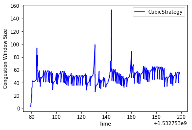
Graph of the congestion window using the CUBIC strategy
Recently, researchers have started using machine learning to address congestion. The general idea is that we can train algorithms that learn from observations in a simulated TCP environments to make decisions about how to change the congestion window. Here, we describe our preliminary attempt at learning from congestion behavior using reinforcement learning, a paradigm in which an agent learns to take optimal actions according to a reward function it has learned from past experience.
Posing Congestion Control as a Reinforcement Learning Problem
Reinforcement learning involves an agent taking actions in some environment. For every action the agent takes, the agent gets some feedback from the environment, which can be interpreted as a reward or penalty, and the “state” of the environment might change For example, for an agent playing Super Mario, the action of gathering coins both changes the state of the environment (there are fewer coins after the action) and rewards the agent by increasing its score. The act of learning to play Super Mario amounts to figuring out what good actions are in a given state, and avoiding bad actions that might end the game early.
While the world of congestion control is decidedly less colorful than that of Super Mario, it can nevertheless be posed in a similar fashion. At each step, a TCP sender needs to make a choice about how to update its congestion window. “Winning” in this world means striking a balance between maximizing throughput and maintaining low per-packet round-trip times.
Reinforcement Learning More Formally
The approach that we take to doing reinforcement learning is called Q-Learning, which involves learning a Q (quality) function that given a state, can provide a “quality” score for each potential action. The quality score takes into account both the immediate reward for taking that action in a given state as well as the future expected reward for the next state that the agent will be in after taking that particular transition.
The reason we want to take the future expected reward into account is so that the agent doesn’t get stuck in a loop where it continues optimizing for some small reward, when it could take an action that might not immediately yield a large reward, but might put the agent in another state where a large reward can be obtained.
This video demonstrates what what happens when an agent gets stuck optimizing for some small immediate reward, rather than actually winning the game.
For a game with a small amount of states and actions, like Tic-Tac-Toe, the Q function can be expressed as a simple table, where the rows correspond to states and the columns correspond to actions that could be taken in each of those states.
Representing the Q Function
For a game with a small amount of states and actions, like Tic-Tac-Toe, the Q function can be expressed as a simple table, where the rows correspond to states and the columns correspond to actions that could be taken in each of those states.
| Action 1 | Action 2 | … | |
|---|---|---|---|
| State 1 | |||
| State 2 | |||
| State 3 | |||
| State 4 | |||
| … |
“Learning” the Q function then, is the process of computing that table.
For games that are more complicated, like Mario or something else that is highly visual, it’s not possible to represent states so simply. If each “state” is a frame in the game, the number of possible game states is really large. The solution to this is to instead approximate the Q function with a neural network.
One of the most well-known uses of neural networks is for image classification. It turns out that this task isn’t that different. Rather than providing the neural network and having it spit out a classification, we now want to provide the neural network with a game state and have it spit out Q values for each of the possible actions at that state.
Mapping RL Concepts to Congestion Control
So, how do we use this to improve congestion control?
In order to pose congestion control as a reinforcement learning properly, we need to define a “state”, what the possible “actions” are, and what the reward function is.
As the state, we use the history of per-packet round trip times. The reason for this is that the decision as to whether we want to increase or decrease the congestion window depends on whether or not the link is congested. The best proxy that a TCP sender has as to whether or not congestion is happening is whether round trip times are increasing relative to some measured base round trip time. This is because an increase in round trip times probably indicates that a queue is building at some router between the sender the receiver of the packets. So if round trip times are higher, the Q function can take this into a account to determine the best next move.
Actions are a little simpler–on receiving acknowledgements from the receiver, the TCP sender needs to decide to either increase the window size, decrease the window size, or keep it the same. This is a rough description, a more rigorous description of these is described in the “Results” section.
The reward function is trickier–but the approach that we’re taking is that if the sender increases the window, and that increase increases the round trip time (a proxy for congestion being caused) over some threshold, the agent receives a negative reward, while if it increases the window without causing a big increase in RTT, it receives a positive reward. This function rewards the agent for increasing the window up to the point that it starts causing RTTs to increase.
Training the Q Function
Now that we’ve defined congestion control as a reinforcement learning problem, the next step is figuring out how to to train the neural network that we’re using.
Since our state, which is a history of round trip times on a link, is a sequence of data points, we use a neural network called an LSTM, which is designed for making predictions based on sequences of data.
To train this LSTM to produce appropriate actions based on sequences of round trip times, we run a series of episodes, in which each episode runs for a minute and involves a sender sending packets constantly to a receiver. The sender has a congestion window set to 1 initially, and will receive acknowledgements from the receiver. Every time an acknowledgement is received, the sender selects an action to take, and adjusts the congestion window accordingly. Also, after making a decision, we track the impact of that decision on the round trip times, and give the agent a corresponding reward. Every time a reward is made, we add that transition to a list of transitions. Note that a transition includes:
- The current state
- An action
- The resulting state
- A reward
We then also optimize the neural network by pulling a random batch of transitions and training the network on those transitions.
In early episodes, the network doesn’t have much experience to draw on, so the agent makes decisions pretty randomly. However, as after the the model has been optimized many times, it begins to be able to make more intelligent decisions.
Some preliminary results
In our preliminary experiments, while the algorithm did not perform better than traditional algorithms like CUBIC, the default in Linux, we did see evidence of learning, and hypothesize that with a higher number of episodes, we could start to see comparable behavior.
In our first experiments, we based our actions on CUBIC: the sender can choose between increasing the window size linearly, or according to a cubic function. Other actions include setting
There are a number of hyperparameters to our model as well. In addition to the configuration of the neural network itself, for instance, the number of hidden layers that we use, the hyperparameters include episode length, the number of historical round-trip times we track in the state, and some other factors about our training.
So, wthout further ado, the results:
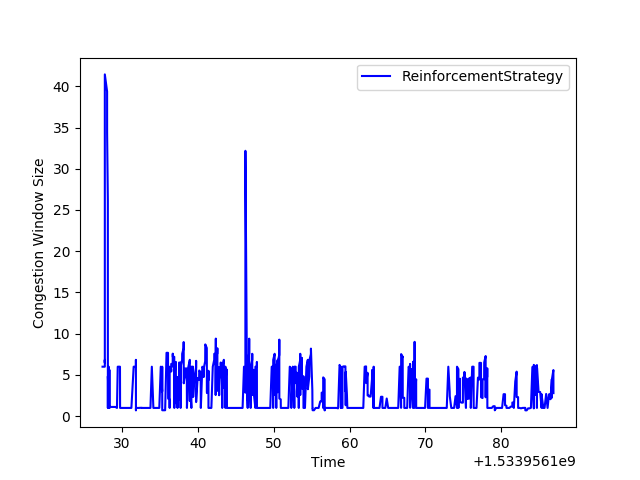
On the first episode of our training, we can see the congestion window moving around pretty randomly as the algorithm selects actions randomly:
By episode 100, we start to see behavior that looks more like the CUBIC graph, (see the graph above for the comparison) and performance that is far superior the original example.
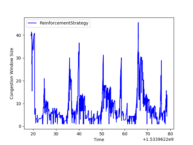
By episode 265, the behavior starts looking pretty good!
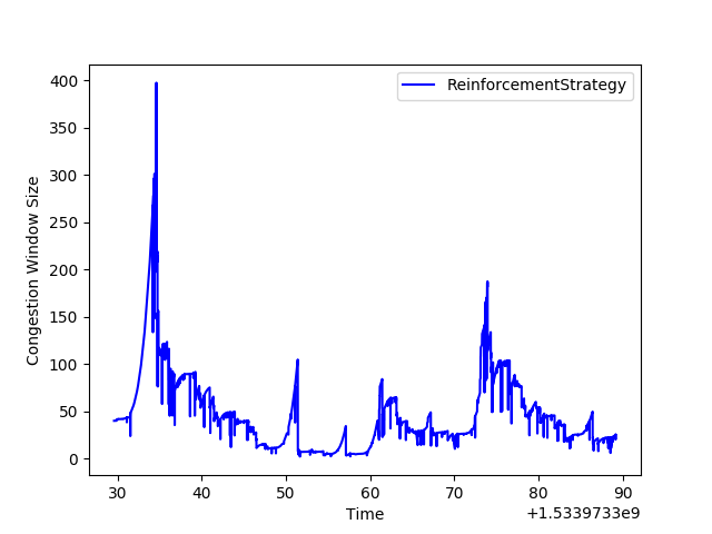
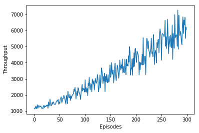
Graphing the throughput over episodes, we see that even by episode 300, the line of best fit is still increasing, suggesting that convergence hasn’t happened yet, and that with more training, we might see results more in line with or better than traditional algorithms.
Conclusion
Reinforcement learning is really powerful and even with the small amount of training we’ve done so far, we’re able to see that the algorithm has learned a strategy to deliver high throughput.
In future experiments, we are going to experiment with changing the configuration of our neural networks and reward functions. Since in the experiment we ran there wasn’t a clear convergence–it’s also clear that we need to run this for a longer period of time.
Learn More
To learn more about congestion control, we’d recommend reading the previous posts on the topic:
For resources on reinforcement learning, we’d recommend:
To better understand LSTMs, the Unreasonable Effectiveness of Recurrent Neural Networks is a great place to start.
We also drew on the work done in Pantheon, in which researchers apply imitation learning to the problem of congestion control (more detail in this paper.
Thanks for reading!