This summer, I’ve been working on coming up with better ways to solve network congestion on the internet. In this post, I’m going to talk about why congestion happens and some traditional solutions.
If you’re interested in a little bit more depth, this Jupyter notebook contains the code that I used to get some of the results, along with further analysis of those results.
What is TCP?
Before we start, I’m going to give a little bit of detail about how information moves around on the internet.
TCP is a protocol that is used to transmit information from one computer on the internet to another, and is the protocol I’ll be focused on in this post. What distinguishes TCP from other networking protocols is that it guarantees 100% transmission. This means that if you send 100kb of data from one computer to another using TCP, all 100kb will make it to the other side.
This property of TCP is very powerful and is the reason that many network applications we use, such as the web and email are built on top of it.
The way TCP is able to accomplish this goal of trasmitting all the information that is sent over the wire is that for every segment of data that is sent from party A to party B, party B sends an “acknowledgement” segment back to party A indicating that it got that message.
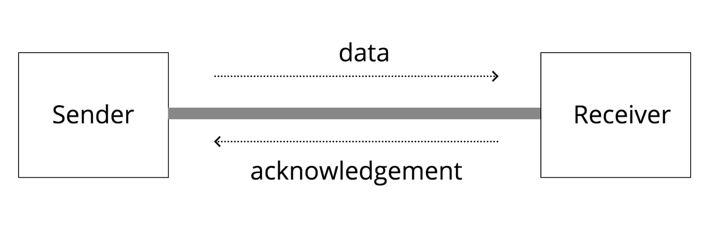
It’s worth noting too that the protocol that TCP works on top of, IP, operates by transmitting packets with a maximum size of 1500 bytes. So if a sender needs to send 100kb, they need to chop up that data into segments, send them over TCP, and receive acknowledgements for all of those segments.
If a sender does not receive acknowledgements from the receiver for a given segment, it will have to resend that segment.
When does congestion happen?
Congestion is problem in computer networks because at the end of the day, information transfer rates are limited by physical channels like ethernet cables or cellular links, and on the internet, many individual devices are connected to these links.
This is a classic case:
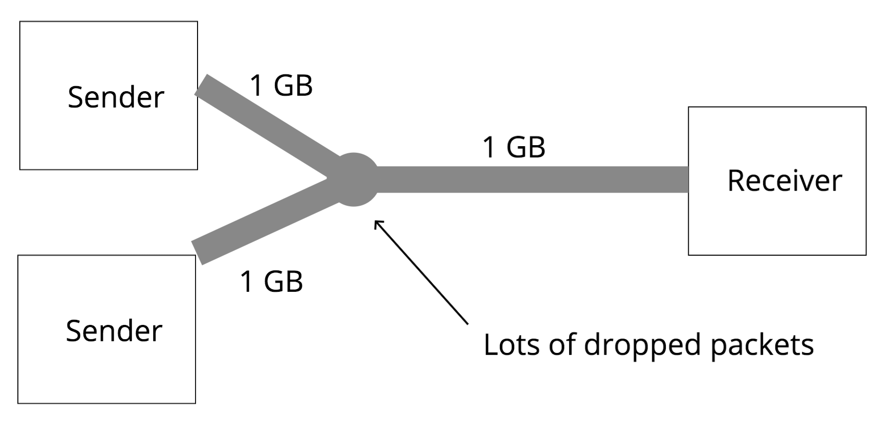
In this picture, two senders are sending information over 1GB links, which both funnel into another 1GB link. The second link cannot accomodate all of the traffic from the two links that funnel into it, and will have to drop some packets. If the senders don’t reduce the amount of information they are each sending, this is going to result in a pretty bad situation. In TCP, if the sender detects that a segment is dropped, it resends that segment, so the congestion will continue, and it’ll take forever for both senders to finish.
In order for both senders to finish sending the information that they are sending, they need to collectively reduce the amount of information that they are sending. In this scenario, if only one sender reduces the amount of information they send and other sender maintains sending 1GB over the wire, congestion will still happen. There isn’t any central system on the internet that can tell the senders exactly what rate that they should be sending at.
Detour: What is a link?
Before I dive into what some solutions to this problem are, I want to be a little bit more specific about the properties of links. There are three important details to know about a link:
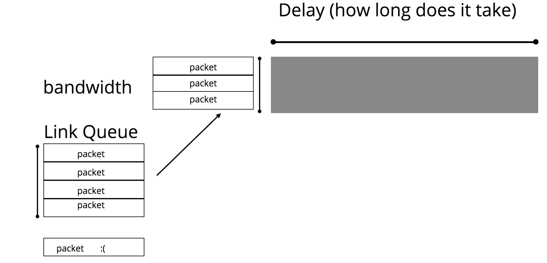
- delay (milliseconds) - the time it takes for one packet to get from the beginning to the end of a link
- bandwidth (megabits/second) - the number of packets that can get through the link in a second
- queue - the size of the queue for storing packets waiting to be sent out if a link is full, and the strategy for managing that queue when it hits its capacity
Using the analogy of the link as a pipe, you can think of the delay as the length of the pipe, and the bandwidth as the circumference of the pipe.
An important statistic about a link is the bandwidth-delay product (BDP). This is a product of the bandwidth and the delay, and is the number of bytes that can fit on the link at any given point in time. This can be thought of the volume of the pipe in the pipe analogy. A link is fully utilized when the number of bytes flowing through it is equal to the BDP. If senders are sending more bytes than the BDP, the link’s queue will fill and eventually start dropping packets.
Approaches
Before diving into solutions, what indicators do senders have that congestion is happening? As I mentioned earlier, the internet is a decentralized system, and as a result of that, doesn’t have any central coordinator telling senders to slow down if link queues downstream of some sender are filling up.
There are two main indicators: packet loss and increased round trip times for packets. When congestion happens, queues on links begin to fill up, and packets get dropped. If a sender notices packet loss, it’s a pretty good indicator that congestion is occuring. Another consequence of queues filling up though is that if packets are spending more time in a queue before making it onto the link, the round trip time, which measures the time from when the sender sends a segment out to the time that it receives an acknowledgement, will increase.
While today there are congestion control schemes that take into account both of these indicators, in the original implementations of congestion control, only packet loss was used.
It’s also worth noting here that senders do not know up front what the properties of the links that they are sending information on are. If you request the website “http://www.google.com”, for instance, the packets you send are probably going through many links before finally getting to Google’s servers, and the rate at which you can send information is fundamentally going to be clamped by the slowest link on that route.
Therefore, in addition to being able to avoid congestion, congestion control approaches need to be able to “explore” the available bandwidth.
The Congestion Window
A key concept to understand about any congestion control algorithm is
the concept of a congestion window. The congestion window refers to
the number of segments that a sender can send without having seen an
acknowledgment yet. If the congestion window on a sender is set to 2,
that means that after the sender sends 2 segments, it must wait to
get an acknowledgment from the receiver in order to send any more. The
congestion window is often referred to as the “flight size”, because it
also corresponds to the number of segments “in flight” at any given point in time.
The higher the congestion window, more packets you’ll be able to get across to the receiver in the same time period. To understand this intuitively, if the delay on the network is 88ms, and the congestion window is 10 segments, you’ll be able to send 10 segments for every round trip (88*2 = 176 ms), and if it’s 20 segments, you’ll be able to send 20 segments in the same time period.
Of course, the risk with raising the congestion window too high is that it will lead to congestion. The goal of a congestion control algorithm, then, is to figure out the right size congestion window to use.
From a theoretical perspective, the right size congestion window to use is the bandwidth-delay product of the link, which as we discussed earlier is the full capacity of the link. The idea here is that if the congestion window is equal to the BDP of the link, it will be fully utilized, and not cause congestion.
TCP Tahoe
TCP Tahoe is a congestion control scheme that was invented back in the 80s, when congestion was first becoming a problem on the internet. The algorithm itself is fairly simple, and grows the congestion window in two phases.
Phase 1: Slow Start: The algorithm begins in a state called “slow start”.
In Slow Start, the congestion window grows by 1 every time an acknowledgement
is received. This effectively doubles the congestion window on every round trip.
If the congestion window is 4, four packets will be in flight at once, and when
each of those packets is acknowledged, the congestion window will increase by 1,
resulting in a window of size 8. This process continues until the congestion
window hits a value called the “Slow Start Threshold” ssthresh. This is
a configurable number.
Phase 2: Congestion Avoidance: Once the congestion window has hit the ssthresh,
it moves from “slow start” into congestion avoidance mode. In congestion avoidance,
the congestion window increases by 1 on every round trip. So if the congestion window is
4, the window will increase to 5 after all four of those packets in flight have been
acknowledged. This increases the window much more slowly.
If Tahoe detects that a packet is lost, it will resend the packet, the slow start threshold is updated to be half the current congestion window, the congestion window is set back to 1, and the algorithm goes back to slow start.
Detecting Packet Loss & Fast Retransmit
There are two ways that a TCP sender could detect that a packet is lost.
-
The sender “times out”. The sender puts a timeout on every packet that is sent out into the wild, and when that timeout is hit without that packet having been acknowledged, it resends the packet and sets the congestion window to 1.
-
The receiver sends back “duplicate acks”. In TCP, receivers only acknowledge packets that are sent in order. If a packet is sent out of order, it will send out an acknowledgement for the last packet it saw in order. So, if a receiver has received segments 1,2, and 3, and then receives segment #5, it will ack segment #3 again, because #5 came in out of order. In Tahoe, if a sender receives 3 duplicate acks, it considers a packet lost. This is considered “Fast Retransmit”, because it doesn’t wait for the timeout to happen.
Some Thoughts
In the Jupyter notebook I talk about earlier, I implemented Tahoe. Here’s a graph of the congestion window over time:
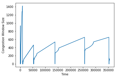
Notice that it has a saw-tooth behavior. The intial spikiness is the slow-start phase, while the smoother parts correspond to congestion avoidance. The sharp drops back down to 1 are due to packet loss.
Why does Tahoe operate like this?
The reason why Tahoe needs to keep growing is that it’s possible for network conditions to change over time. For instance, if another sender starts sending packets on the same link, it will reduce the bandwidth available, and the sender will need to adjust accordingly. If another sender on the same link stops sending packets, the sender will have more bandwidth available, and in order to utilize it, will need to adjust accordingly.
There are a number of issues with this approach though, which is why it is no longer used today. In particular, it takes a really long time, especially on higher bandwidth networks, for the algorithm to actually take full advantage of the available bandwidth. This is because the window size grows pretty slowly after hitting the slow start threshold.
Another issue is that packet loss doesn’t necessarily mean that congestion is occuring–some links, like WiFi, are just inherently lossy. Reacting drastically by cutting the window size to 1 isn’t necessarily always appropriate.
A final issue is that this algorithm uses packet loss as the indicator for whether there’s congestion. If the packet loss is happening due to congestion, you are already too late–the window is too high, and you need to let the queues drain.
Other approaches
Since the 80s, a number of algorithms have been developed that take some of these issues into account. I will explore some of these in more detail in future blog posts!
CUBIC: This algorithm was implemented in 2005, and is currently the default congestion control algorithm used on Linux systems. Like Tahoe, it relies on packet loss as the indicator of congestion. However, unlike Tahoe, it works far better on high bandwidth networks, since rather than increasing the window by 1 on every round trip, it uses, as the name would suggest, a cubic function to determine what the window size should be, and therefore grows much more quickly.
BBR (Bufferbloat): This is a very recent algorithm developed by Google, and unlike Tahoe or CUBIC, uses delay as the indicator of congestion, rather than packet loss. The rough thinking behind this is that delays are a leading indicator of congestion–they occur before packets actually start getting lost. Slowing down the rate of sending before the packets get lost ends up leading to higher throughput.
Fairness
A fascinating issue to consider with different congestion control schemes is whether or not certain schemes are “fair” to other TCP senders on the same link. A scheme would be unfair to other senders if during times of congestion it, rather than also scaled back, continued to send at the same rate. I include here the results when a sender without congestion control is running on the same link as a sender using Tahoe. As you can see here, in a one minute period, the Tahoe sender barely gets any bytes through, because it doesn’t get a chance to increase its window much at all, while the fixed window sender just blasts the network with packets.
While the Fixed Window Sender is a particularly bad case, it is possible for algorithms to be unfair and grow to use more bandwidth than other algorithms. Since there isn’t a central controller responsible for telling senders what to do, it is totally possible for a single sender to be greedy, and as a result there’s a game theortic angle to congestion control too.
Conclusion
Congestion control is a fundamental feature of the internet and is a fascinating exercise in distributed decision making with limited information.
Again, if you’re interested in seeing more details about the experiments I ran, check out my Jupyter Notebook.
Over the next few weeks, I’m going to be working on implementations of other congestion control algorithms, and hopefully make some progress on a machine learning- based congestion control approach. Stay tuned!