In my last post, I introduce the problem of congestion control in computer networks, and one of the early solutions to it, Tahoe.
In this post, I’m going to cover a different and more modern approach, CUBIC, which is the default TCP in most Linux distributions today. If you’re interested in the details of the experiments I ran, check out this Jupyter notebook.
But first, a recap
Congestion on the internet happens when the computers send more packets to a particular link than that link can handle. If a link is receiving more packets than can fit on the wire, it will begin queueing up those packets, and if the link’s queues fill up, the link will begin dropping those packets.
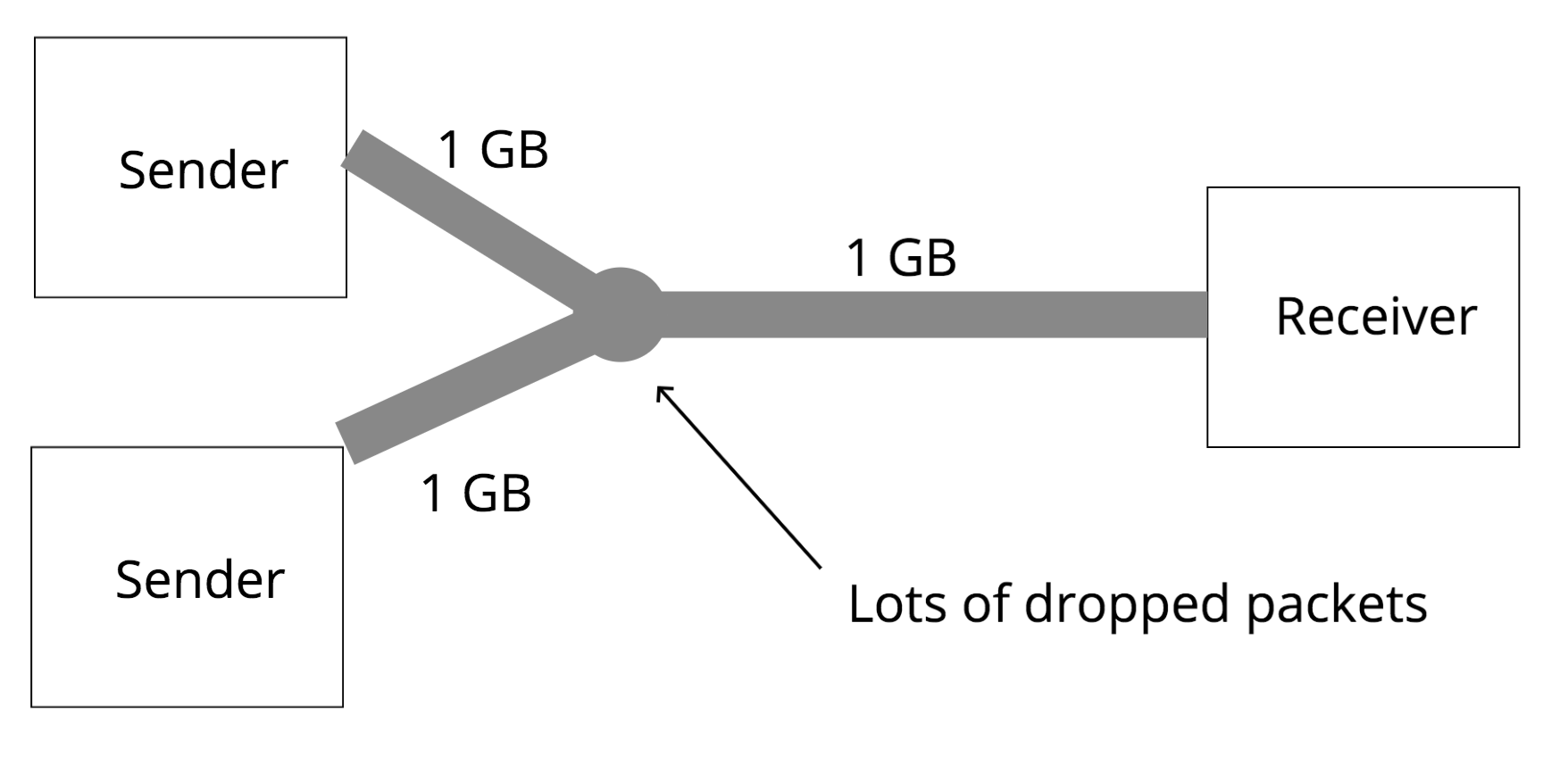
Why can’t senders just send packets at a rate the link can handle?
Another big problem that TCP encounters is that senders don’t actually know the available bandwidth on the particular path they sending on. On certain networks, like cellular networks, the bandwidth and delay times might change fairly frequently depending on where you physically move. Also, even on your home WiFi, somebody else also using the internet might change the available bandwidth.
Computers have no way of knowing when events like this happen. So, in order to effectively use the bandwidth available to them, senders need to constantly increase the amount of packets they send every round trip time to explore that available bandwidth. When they experience drops, they then know what the limits of the current bandwidth are.
Traditional approach
The traditional approaches to congestion control in TCP, named Tahoe and Reno, operate by increasing the congestion window size, which you can think of as the “rate” at which senders send packets, exponentially until some threshold is reached. After that threshold is reached, they begin increasing linearly.
Once they experience drops, they will aggressively drop the window size, and then enter “slow start” mode again, where they increase exponentially until they hit the threshold. Once the threshold is hit, they will increase linearly again.
The internet’s different now!
The approaches Tahoe and Reno were were developed in the late 80s and 90s, and worked then, but the internet has changed a lot since. Notably, there now exist longer, and higher bandwidth networks (long, fat networks). In order to fully take advantage of these networks, TCP senders need to send with much higher congestion windows.
Since Tahoe & Reno grow linearly after crossing the slow start threshold, if a lot more bandwidth becomes available on a link, it’ll take a long time for these algorithms to “discover” that available bandwidth.
Enter: CUBIC
It turns out that in order to achieve better performance on “long, fat networks”, these congestion control algorithms need to do a better job of “exploring” for more bandwidth.
However, we don’t want to overload a network, or aggressively steal away available bandwidth from other senders on the same network.
It turns out that there’s a mathematical function for growing the congestion window that satisfies both of these contraints, the cubic function:
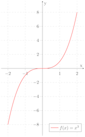
Observe a very powerful property of a cubic function: that as x is lower, t function
grows very quickly, and then slows down as it approaches a particular point (the inflection point), and then
after crossing that point begins growing quickly again.
Why is this useful in congestion control?
It turns out that you can take advantage of this property when designing a congestion control algorithm:
If the congestion window is grown as a cubic function of time since the last packet drop, and the inflection point is set to be the size of the congestion window at the last drop, the window has the following behavior:
- Start growing really fast
- As the algorithm approaches the window at the last drop, the congestion window begins growing more slowly
- If the congestion window gets to the point at which drops occurred the last time, and does not experience a drop, begin growing slowly again, but then increase more quickly
The concave portion of this, where the window begins growing quickly but then slows down, and the convex portion of this can be thought of two different phases. During the concave phase, the congestion window is catching up to where a packet was lost last time, and slows down its growth to be fair to traditional TCP senders. If the algorithm gets there without experiencing drops, it can move into an “exploratory” phase, in which it grows quickly to discover newly available bandwidth.
Results
Alright, so how does CUBIC do in practice? While the full results are here, here are some highlights:
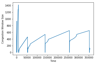
On a 2.64mbps network with an 88ms delay, we see a pretty big increase over Tahoe. Here’s a graph of the congestion window over time:
Notice that the graph of the congestion window behaves like a cubic function. While Tahoe sees a 10.42kbps throughput, CUBIC sees 14.56kbps.
How fair is it?
Let’s next look at how it does when run on the same link as Tahoe:
On a low BDP network:
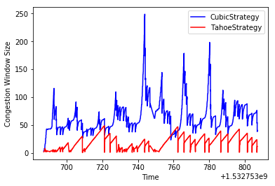
Here we see the Tahoe performance drop to 6.15kbps, and the CUBIC performance increase to 17.50kbps. It’s interesting that CUBIC increases relative to how it performed by itself!
On a high BDP network:
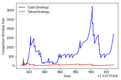
Here, we see that Tahoe doesn’t do very well, getting 6.63kbps, while CUBIC gets 37.7kbps!
Overall, it looks like running CUBIC side-by-side with Tahoe on the same link results in some degradation of performance for Tahoe. However, with some more tuning, and a less aggressive CUBIC algorithm, it’s conceivable that it doesn’t steal away as much of the flow from Tahoe as it does in my simulation. In the paper introducing CUBIC, the experimental results indicate that CUBIC doesn’t detract from the performance of standard TCP.
CUBIC and Queues
One of the interesting results above is that CUBIC actually performs better when running on the same link as another sender than it does when it is sending on its own.
This is an odd result, you’d actually expect the opposite to happen. Why is it that adding another consumer of the link makes a difference?
The answer is to do with how the queues at links react. In the scenario where there are multiple senders on the same link, the link queue actually fills up much faster than in the scenario when CUBIC is sending by itself. This causes CUBIC to back off earlier than when it is the only sender. The earlier correction prevents CUBIC from getting into a state in which the window grows really fast, until the queue fills up, causing a block of packets to get dropped and cause CUBIC to drop its window size a lot. In addition to this, Tahoe backs off much more aggressively than CUBIC, meaning that when loss events occur, CUBIC has even more queue space to use.
If this is confusing, don’t worry–I’ll be fleshing this out in more detail in my next post.
Next Up
CUBIC is a very effective congestion control algorithm, and has been the default congestion control algorithm in Linux since 2006.
However, there are still some problems with it. Notably, the high BDP example in this post suggests that a big queue size can actually cause CUBIC to perform worse. Moreover, since CUBIC doesn’t back off the window size until packet loss occurs, a big queue can mask the fact that the sender’s window is too big, and the growing queue can cause round-trip times to increase.
In my couple posts, I’m going to explore solutions to these problems.