Last week, Lucy Zhang and I worked on compressing images with the Discrete Cosine Transform (DCT).
I was pretty blown away by how well this ended up working, and in this post, I’m going to explain the intuition behind why. If you’re curious about the work that we did, check out our code.
But first, what is compression?
A note on compression
In addition to being a major plot element on HBO’s Silicon Valley, compression is also the process of reducing the amount of space needed to represent data. In practice, that “data” could be text, images, video, audio, or really anything else. There are two main types, lossless, and lossy. In lossless compression, 100% original data can be recovered in the decompression process, while with lossy compression, “uninteresting” pieces of the original data are thrown out, while the important structure is retained. What consitutes “uninteresting” pieces of data is up to the compression algorithm used.
Compression with DCTs is a form of lossy compression–here are our results:
Before:

After:

As you can see, the compressed image is a little fuzzier than the original, but the core features of the image are still recognizable.
Compressed even further:

Because we are using lossy compression, the amount of “loss” we are willing to tolerate is configurable. Here, we compress the image even further. There is a very distracting blur on the image now, and a lot of detail is missing. However, the core structures of the image, like the baboon’s nose and eyes, can still be discerned.
This is pretty incredible. Without our algorithm “knowing” anything about baboons, it was able to “figure out” what the core structures of the image are.
What is a Fourier transform?
The DCT is a a type of Fourier-related transformation. A Fourier transform is the process of decomposing some kind of digital signal into the sum of some trignometric functions.
So for instance, if you have audio signal like the following:
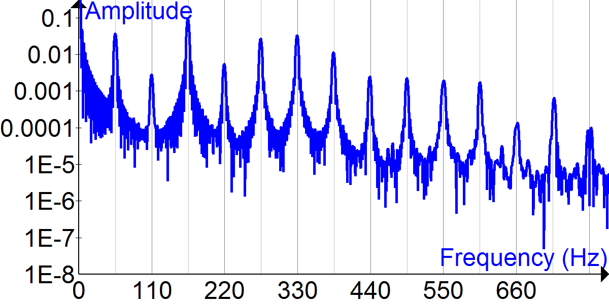 By Fourier1789 [CC BY-SA 4.0 (https://creativecommons.org/licenses/by-sa/4.0)], from Wikimedia Commons
applying a Fourier transform would yield a bunch of different sine and cosine
waves of different frequencies that sum together to be the equivalent of the
original audio wave.
It’s called a transform because it transforms the data from one form, the amplitude over time, into a list of coefficients, where each coefficient corresponds to a different trignometric function and governs “how much” of that function to use in order to get the original wave.
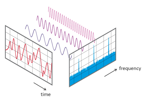
By Phonical [CC BY-SA 4.0 (https://creativecommons.org/licenses/by-sa/4.0)], from Wikimedia Commons
It’s worth noting that these are equivalent ways of encoding the sound wave. This is a fundamental property of Fourier transforms–no data is lost converting between these two “formats” of encoding the data.
What does this have to do with images?
Similarly to audio, image data can also be modeled by waves. Let’s start by understanding how to deal with images as numerical data.
For grayscale images, we can model them as a matrix of values, where the element at position
(i,j) in the matrix corresponds to the pixel at position (i,j) in the image, and the value of
that matrix element is the pixel’s intensity. 0 corresponds to black, and 255 corresponds to white.
It may not be obvious that any image data is “wave-like”, so let’s try graphing some image data!
From the baboon image, let’s take a row of pixels from halfway down the image (it’s 256 pixels long, so this picture is only the first few):
![]()
Graphing the values of an entire row of pixels, we get a picture that looks like this:
![]()
This is pretty cool! Remembering that 255 represents the color white, we get two nice peaks, which represent the nose of the baboon, which has some dark coloring in the middle.
It’s clear from this picture that the pixels follow a wave-like pattern, and it’s not hard to imagine that this could be represented as the sum of some trignometric functions.
What does this have to do with compression?
There are some clues in the graph above as to how figuring out how the decomposition of
that picture into different sine and cosine waves might be useful in compressing the image.
Specifically, it’s clear that some of the structure in the graph is very important to preserve. Notably, it’s very important to preserving the overall structure of the image to preserve the peaks in the middle of the graph, as we’d want any compressed image to still have a nose.
However, some of the higher frequency components, like the smaller changes in amplitude leading up to those peaks, are less important, and could be removed without us losing the notion of a “nose”. Once we have decomposed the image into a bunch of trig functions, it becomes easy to remove higher frequency functions that don’t contribute as much to the core structures of the image. As I mentioned in a previous section, it is a property of Fourier transforms that they are reversable–given the trig functions and the coefficients, the original data can be recovered. So after removing the higher frequency components, a new, compressed image can be generated.
How do we perform the “decomposition”?
That concludes the main intuition behind why breaking down an image in a sum of trignometric function can help in image compression.
The next question, then, is how exactly one goes about decomposing the image data into component trig functions.
The Discrete Cosine Transform
The mechanism that we’ll be using for decomposing the image data into trignometric functions is the Discrete Cosine Transform. In this post, I won’t be going deep into how the math works, and will be a little hand-wavy, so if you’re interested in going further, the wikipedia page is a great starting point.
I’ll start by considering how this would for a single row of pixels.
The DCT is a linear transformation that transforms a vector of length n containing “amplitudes”, and returns a different vector of length n containing the coefficients for n different cosine functions. Therefore, it is encoded by an n x n matrix, in which each row corresponds with a cosine function of a different frequency.
Why use n cosine waves?
An important feature that is required in order for our image compression to work properly
is that the transformation that we use to decompose the data into cosine functions must
be invertible. If used fewer or greater than n cosine functions, then we would not
be able to represent the transformation as a square matrix, and it would therefore not
be invertibile, which is the key to being able to get our data back in terms of amplitudes
after converting it to cosine coefficients.
Generating the cosine functions
Alright, so we know now that the DCT for a length n array of pixels will be represented
by an n x n matrix, where each row in the matrix corresponds to a different cosine wave.
The next question then is how do you represent a cosine wave as a row in a matrix?
If X is the transformation matrix, the matrix values are given by:
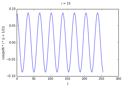
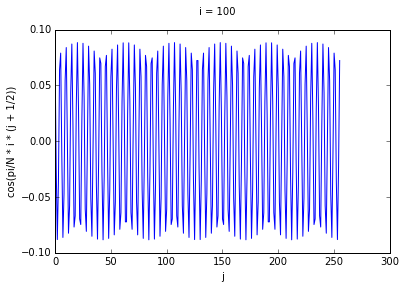
Here, i, indicates the row we are on, and j the column within that row. N is the total size
of the matrix, so both i and j range from 0 to N.
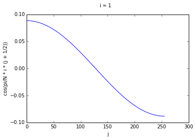
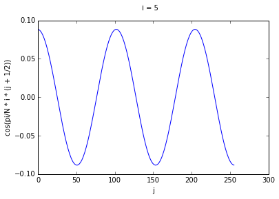
If we think of each row as corresponding to a different cosine function, we can see that higher
values of i correspond to cosine waves of higher frequency. To prove this to ourselves, we can
graph some rows for some values of i.
Performing the decomposition
The next step, after computing the DCT matrix, is actually performing the decomposition and figuring
out the right coefficients for each of the component waves. The short answer here is that this
is a simple matter of matrix multiplication–we take our input vector of pixel intensities ,
and multiply it by X, and get our coefficient vector , where each value in
corresponds to a coefficient.
But what is really happening here? When we perform matrix multiplication we are for each row in X
taking the dot product of and . The dot product can be interpreted as a measure of similarity between two vectors-
-how much of is in ? If the pixel data is coincident with the values
in one particular wave, the value of the dot products, and if it is orthogonal, it will
be 0. Therefore, by computing this dot product, we can figure out what coefficient
to use for that particular wave.
Generalizing this to two dimensions
Great, so now we can get our decomposition for a single row of pixels. Alas, single rows of pixels tend to not be super interesting, how do we get this to work in two dimensions?
The naive solution is to just apply this transform for each row of pixels. However, the issue with this is that there is signal and structure in the columns that we miss if we don’t take that into account. This can be remedied by performing the DCT twice–once along the rows, and then again along the columns.
Performing the compression
Once we’ve computed the DCT transform in two dimensions, what we’re left with is an n x n
matrix–with each value in the matrix corresponding to the coefficient of a cosine function,
rather than the amplitude values of the original matrix.
Let’s say the original resolution of the image is 256 x 256 pixels. This means that the DCT transform matrix will have dimensions of 256 x 256. The way the compression works is that you take the K most signalful cosine waves, and save the coefficients for those to disk. Say, for instance, we choose to save the coefficients for 100 functions. What we end up saving to disk is a 100 x 100 matrix, instead of the full uncompressed 256 x 256 matrix.
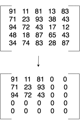
A 5x5 DCT matrix compressed to 3x3
When we want to read the file back off the disk, pad the matrix with 0’s to get a 256 x 256 matrix, and then put it through the inverse DCT to get the compressed image.
What one chooses to compress to completely depends on the application and use case for the
compression. The tradeoff for different sizes of K is that with higher values of K, the
quality of the image will be higher, while for lower values, the size on disk will be lower.
Why the DCT?
The DCT is only one of many Fourier-related transforms, each of which decomposes a signal into the sum of different combinations of sine and cosine wave. It’s worth noting that image compression can be done with other types of transforms, for instance, the Discrete Fourier Transform (DFT).
The main difference between the DCT and DFT is that the DFT does not just use cosine waves–the waves that it uses are a combination of sine and cosine waves. I’m not going to get into the details as to why here, but in practice, the DCT typically allows for more signal to be retained with fewer functions.
Final Thoughts
I hope that you are as blown away by the power of the DCT as me. If you’re curious about digging more deeply into the math behind the DCT, and proving to yourself the statements that I waved my hands over, I’d highly recommend the wikipedia page as a good starting point.
My biggest takeaway from this exercise is how incredible it is that a fairly simple math operation can be used to used to discern major features from an image. And even more impressive is that the DCT can be used to store the image in a more semantically meaningful way that in an array of pixels–it can actually be stored in a way that encodes information about broader structures of the image. I’m very curious now as to whether this kind of encoding is used to prepare data for machine learning algorithms.
I’d like to also thank Lucy again for introducing me to this topic and for working on this project with me.